BKMR-CMA Effect Of Joint Exposures when the Effect Modifier is Fixed
Source:vignettes/BKMRCMA_Effectof_singleZ.Rmd
BKMRCMA_Effectof_singleZ.RmdIn this scenario, we have a continuous mediator
,
a continuous outcome
,
and x2 as the effect modifier on
.
The sample size is 50 and there are 3 covariates.
We can generate a basic sample dataset analogous to the one presented in the QuickStart guide and proceed to fit the BKMR models in the same way.
Joint effect of co-exposure to Z1, Z2 and Z3 and single variable effects, presented when the effect modifier is fixed at its 10th percentile or 90th percentile
list.fit.y.TE <- list(fit.y.TE)
colnames(list.fit.y.TE[[1]]$Z) <- c("z1", "z2", "z3", "E.Y")


overallrisks.y.TE.joint.x10 <- OverallRiskSummaries.MI(list.fit.y.TE, qs = seq(0.1, 0.9, by = 0.05), q.fixed = 0.5, q.alwaysfixed = 0.1, index.alwaysfixed = 4, sel = sel, method="approx")

overallrisks.y.TE.joint.x90 <- OverallRiskSummaries.MI(list.fit.y.TE, qs = seq(0.1, 0.9, by = 0.05), q.fixed = 0.5, q.alwaysfixed = 0.9, index.alwaysfixed = 4, sel = sel, method="approx")
pA <- ggplot(overallrisks.y.TE.joint.x10, aes(quantile, est, ymin = est - 1.96*sd, ymax = est + 1.96*sd)) +  geom_hline(yintercept=00, linetype="dashed", color="gray")+
  geom_pointrange(size = 0.1)+ ggtitle("A")+ scale_y_continuous(name="estimate", limits = c(-1.3, 1.8)) + theme(axis.title = element_text(size = 6), axis.text = element_text(size = 5))

pB <- ggplot(overallrisks.y.TE.joint.x90, aes(quantile, est, ymin = est - 1.96*sd, ymax = est + 1.96*sd)) +  geom_hline(yintercept=00, linetype="dashed", color="gray")+
  geom_pointrange(size = 0.1)+ ggtitle("B")+ scale_y_continuous(name="estimate", limits = c(-1.3, 1.8)) + theme(axis.title = element_text(size = 6), axis.text = element_text(size = 5))
ggarrange(pA , pB , ncol=2, nrow =1)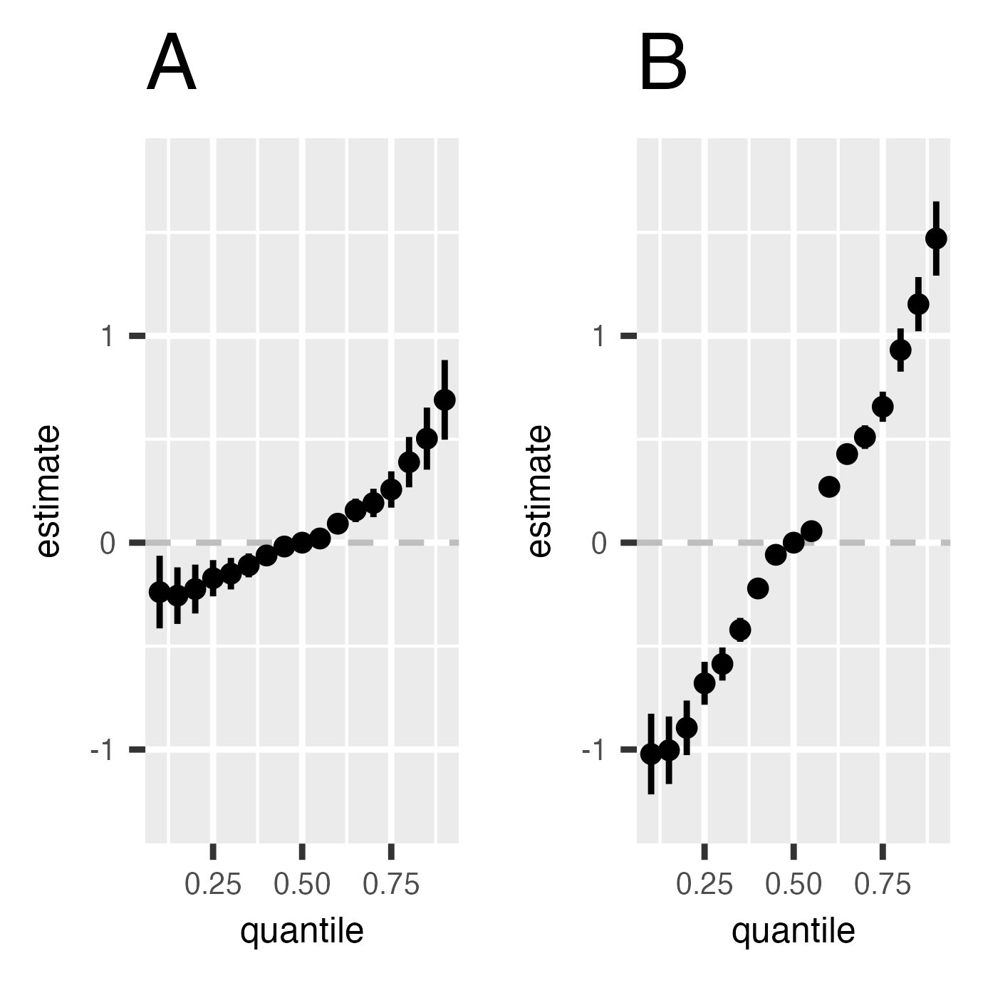
Interpretation of the point estimate in figures A, B:
Figure (A). Overall effect of the mixture (estimates and 95% credible
interval) , by comparing the value of h when all of
predictors are at a particular percentile as compared to when all of
them are at their 50th percentile, while the effect modifier
E.Y is fixed at it’s 10th percentile.
Figure (B). Overall effect of the mixture (estimates and 95% credible
interval) , by comparing the value of h when all of
predictors are at a particular percentile as compared to when all of
them are at their 50th percentile, while the effect modifier
E.Y is fixed at it’s 90th percentile.
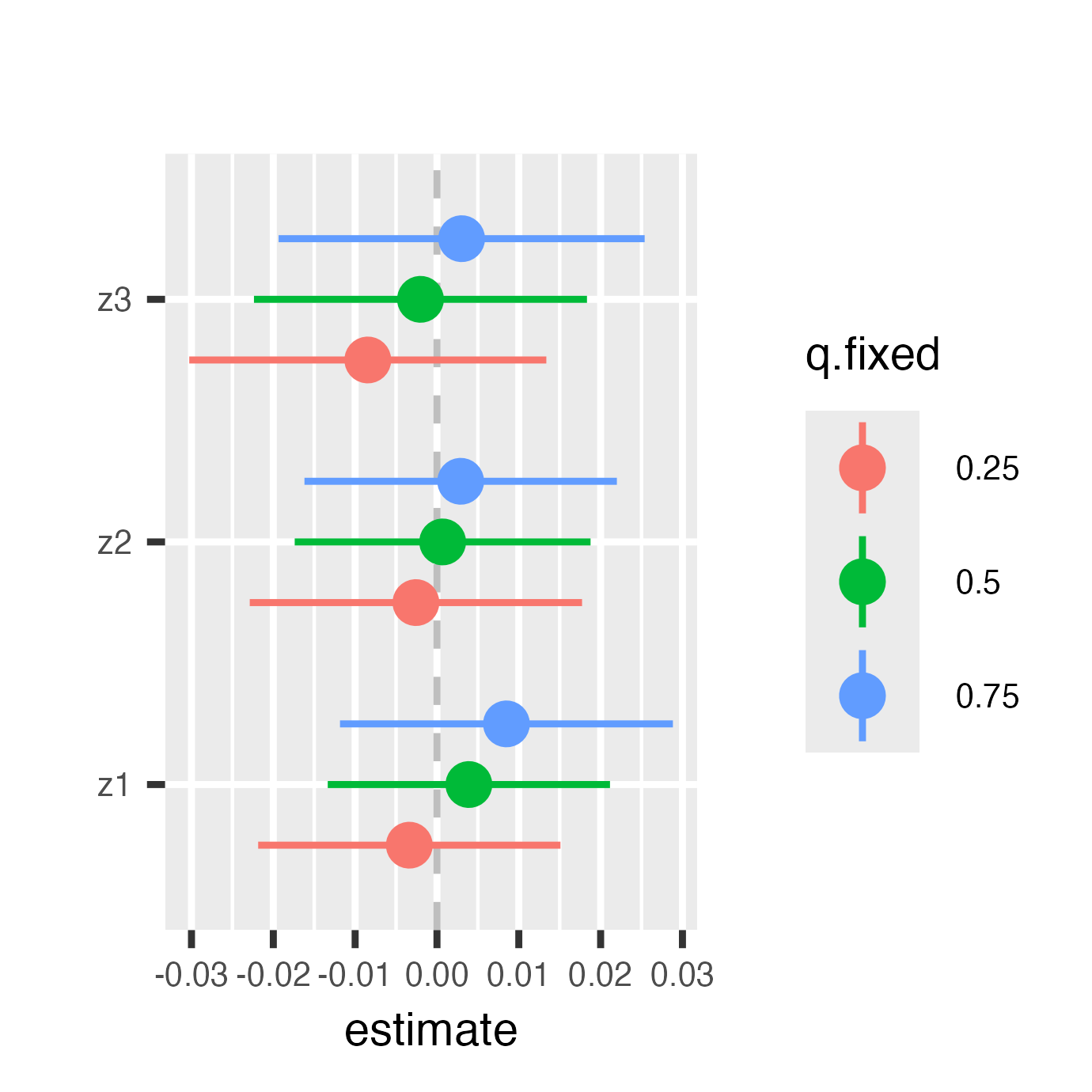
Single exposure associations with outcome Y (estimates and 95% CI) presented when the effect modifier is fixed at its 90th percentile
singvarrisk.y.TE.joint.x90 <- SingVarRiskSummaries.MI(list.fit.y.TE, which.z=c(1,2,3), qs.diff = c(0.25, 0.75), q.fixed = c(0.25, 0.50, 0.75), q.alwaysfixed = 0.9, index.alwaysfixed = 4, sel=sel, method = "approx")
pD <- ggplot(singvarrisk.y.TE.joint.x90 , aes(variable, est, ymin = est - 1.96*sd,  ymax = est + 1.96*sd, col = q.fixed)) +  geom_hline(aes(yintercept=0), linetype="dashed", color="gray")+
  geom_pointrange(position = position_dodge(width = 0.75)) +  coord_flip() + ggtitle("")+
  scale_x_discrete(name="")+ scale_y_continuous(name="estimate") + theme(axis.title = element_text(size = 7), axis.text = element_text(size = 6), legend.title = element_text(size = 7), legend.text = element_text(size = 5))
pD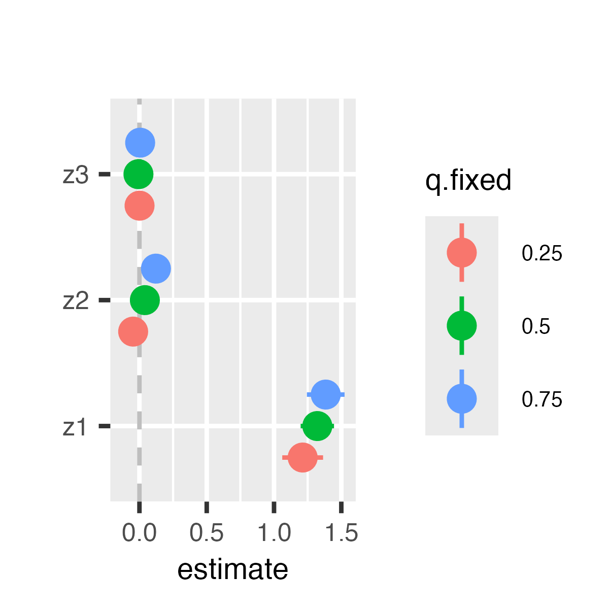
Interpretation of the point estimate in the figure:
:
:
:
The figure represents the single exposure association (estimates and
95% credible intervals) while the effect modifier E.Y is
fixed at its 90th percentile. This plot compares the outcome when a
single exposure is at the 75th vs. 25th percentile, and the effect
modifier is fixed at its 90th percentile.
Functions for the scenarios where multiple Exposures are presented
In the follwing scenario, we have a continuous mediator
,
a continuous outcome
.
x1 and x2 are both effect modifiers on
.
The sample size is 50 and there are 3 covariates.
dat <-  cma_sampledata(N = 50, L=3, P=3, scenario=5, seed=7)
head(dat$data, n = 3L)
dat = dat$data

A <- cbind(dat$z1, dat$z2, dat$z3)
X <- cbind(dat$x1, dat$x2, dat$x3)
y  <- dat$y
m  <- dat$M

E.M <- NULL
E.Y <- cbind(dat$x1, dat$x2)

Z.M <- cbind(A,E.M)
Z.Y <- cbind(A, E.Y)
Zm.Y <- cbind(Z.Y, m)

set.seed(2)
fit.y.TE <- kmbayes(y=y, Z=Z.Y, X=X, iter=10000, verbose=TRUE, varsel=FALSE)
#save(fit.y.TE,file="bkmr_y_TE.RData")

X.predict <- matrix(colMeans(X),nrow=1)
sel<-seq(5000,10000,by=10)

list.fit.y.TE <- list(fit.y.TE)
colnames(list.fit.y.TE[[1]]$Z) <- c("z1", "z2", "z3", "x1", "x2")
Overall Risk Summaries for a list of fixed percentiles of the Effect modifiers
By using the OverallRiskSummaries.fixEY function, we can
specify what is the set of effect modifiers, and what percentiles we
want them to be fixed at. For the following example, x1 and
x2 are specified as the effect modifiers, and the following
code estimates the joint effect of the set of exposures
(i.e. z1, z2, and z3), while the
set of effect modifiers are fixed at the 85th percentile.
ListofResTables <- OverallRiskSummaries.fixEY(list.fit.y.TE, qs = seq(0.1, 0.9, by = 0.05),
                           q.fixed = 0.5, q.alwaysfixed =  c(0.15, 0.85),
                           EY.alwaysfixed.name =  c("x1", "x2"), sel = sel, method="approx")
#ListofResTables[[2]] is the summary of the joint effect of the exposures when the set of effect modifiers are fixed at 85th percentile

pF <- ggplot(ListofResTables[[2]], aes(quantile, est, ymin = est - 1.96*sd, ymax = est + 1.96*sd)) +
  geom_hline(yintercept=00, linetype="dashed", color="gray")+
  geom_pointrange()+ scale_y_continuous(name="estimate")  + theme(axis.title = element_text(size = 7))
pF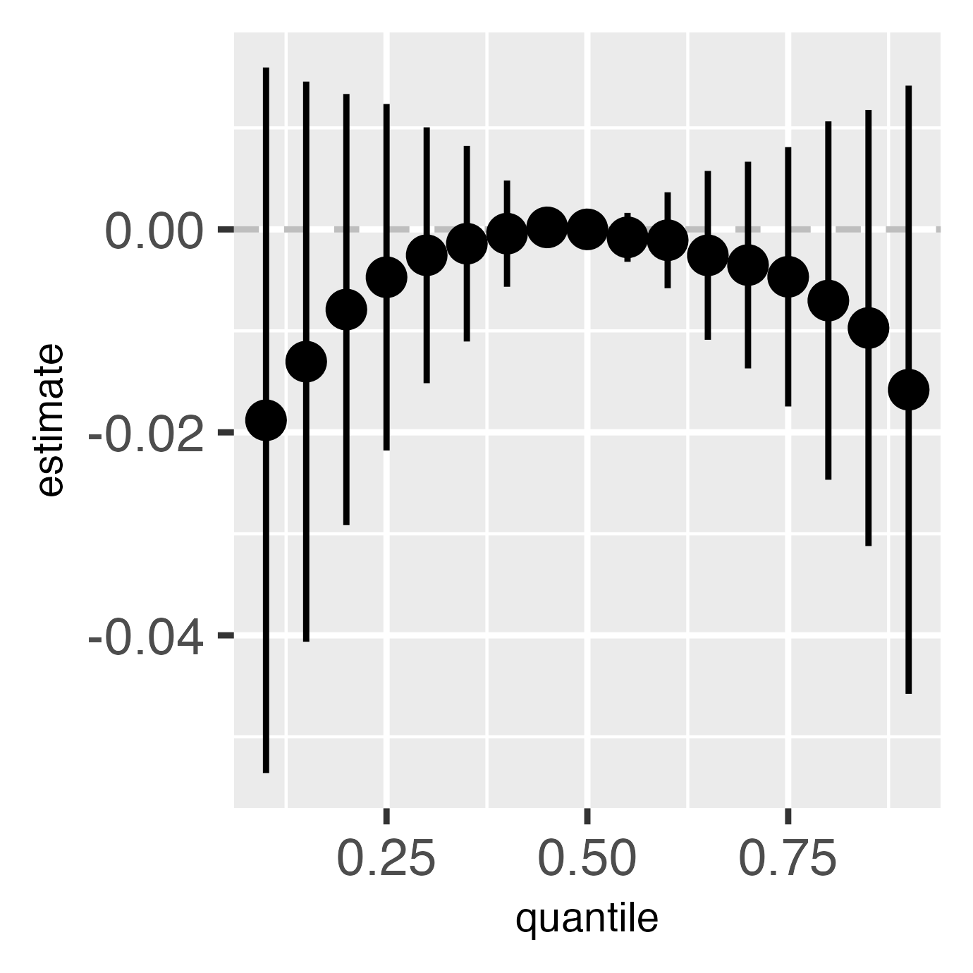
Single Variable Risk Summaries for a list of fixed percentiles of the Effect modifiers
By using the OverallRiskSummaries.fixEY function, we can
specify what is the set of effect modifiers, and what percentiles we
want them to be fixed at. For the following example, x1 and
x2 are specified as the effect modifiers, and the following
code compares the outcome when a single exposure is at the 75th vs. 25th
percentile, when all the other exposures are fixed at either the 25th,
50th, or 75th percentile, while the set of effect modifiers are fixed at
the 85th percentile.
ListofResTablesSingvar <- SingVarRiskSummaries.fixEY(list.fit.y.TE, which.z = c(1,2,3), qs.diff = c(0.25, 0.75),
                                                     q.fixed = c(0.25, 0.50, 0.75),
                                                     q.alwaysfixed = c(0.15, 0.85), z.names = c("z1", "z2", "z3"),
                                                     EY.alwaysfixed.name =  c("x1", "x2"), sel = sel, method="approx")
#> [1] "1 out of 3 complete:  0 min run time"
#> [1] "2 out of 3 complete:  0 min run time"
#> [1] "3 out of 3 complete:  0 min run time"
#> [1] "1 out of 3 complete:  0 min run time"
#> [1] "2 out of 3 complete:  0 min run time"
#> [1] "3 out of 3 complete:  0 min run time"
#ListofResTablesSingvar[[2]]
#ListofResTablesSingvar[[2]]

pH <- ggplot(ListofResTablesSingvar[[2]] , aes(variable, est, ymin = est - 1.96*sd,  ymax = est + 1.96*sd, col = q.fixed)) +
  geom_hline(aes(yintercept=0), linetype="dashed", color="gray")+
  geom_pointrange(position = position_dodge(width = 0.75)) +  coord_flip() + ggtitle("")+
  scale_x_discrete(name="")+ scale_y_continuous(name="estimate") + theme(axis.title = element_text(size = 7), axis.text = element_text(size = 5), legend.title = element_text(size = 7), legend.text = element_text(size = 5))
pH